
Diffraction Anisotropy Server
Perform Ellipsoidal Truncation and Anisotropic Scaling
New JobDiscussion of Your Results
| Background | |||||
 What is diffraction anisotropy?
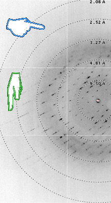
Diffraction anisotropy is evidenced as a directional dependence
in diffraction quality. For example, in the diffraction
pattern on the right, the crystal diffracts to higher resolution in
the horizontal direction (green pointer) than in the vertical direction
(blue pointer). Diffraction anisotropy is commonly observed in protein
crystallography, ranging from moderate to severe. It is attributed
to whole-body anisotropic vibration of unit cells, for example crystal
packing interactions being more uniform in one direction than another.
Frequently, the directional dependence coincides with reciprocal cell
directions a*, b*, and c*.
What is diffraction anisotropy?
Diffraction anisotropy is evidenced as a directional dependence
in diffraction quality. For example, in the diffraction
pattern on the right, the crystal diffracts to higher resolution in
the horizontal direction (green pointer) than in the vertical direction
(blue pointer). Diffraction anisotropy is commonly observed in protein
crystallography, ranging from moderate to severe. It is attributed
to whole-body anisotropic vibration of unit cells, for example crystal
packing interactions being more uniform in one direction than another.
Frequently, the directional dependence coincides with reciprocal cell
directions a*, b*, and c*. Can diffraction anisotropy impede crystallographic refinement? Moderate cases of diffraction anisotropy are adequately handled by automatically applied anisotropic scaling algorithms such as those applied in REFMAC or CNS. But, when the directional dependence in resolution becomes strong or severe, refinement can stall at high R-factors and electron density maps can appear featureless, thus inhibiting model building efforts. In the case cited above (Strong et al., 2006), the difference between the best and worst diffracting directions of the crystal were 2.3 and 3.3 Angstroms, respectively. R-factors were stalled at Rwork=38.5%, Rfree=43.4%. One of the frames from the data set is pictured on the right. How does diffraction anisotropy stall improvement of the R-factor? There are two means by which anisotropy impacts the R-factor. The first has to do with the inclusion of numerous poorly measured reflections in anisotropic data sets (i.e. F/sigma less than 3.0). Because they make up a considerable fraction of the data set, the R-factor in anisotropic refinement tends to be high. Inclusion of these weak reflections is a consequence of the shortcomings of currently available data processing programs such as Denzo and Mosflm. If one wishes to include all the reflections in the well diffracting direction, one is forced to also include the reflections in the weak diffracting direction as well. In other words, the resolution cutoff for a data set processed by Denzo or Mosflm is spherical, whereas the intensity of the difraction pattern is ellipsoidal. The solution to this aspect of the problem is to impose an ellipsoidal resolution boundary on the data, rather than a conventional spherical boundary, so that the weak reflections falling outside the ellipsoidal boundary are removed from the data set and from the refinement process. This procedure is called ellipsoidal truncation. It differs from the conceptually simpler (and less desirable) procedure of imposing an F/sigma cutoff in the refinement program. Both procedures remove weak reflections from the data set, but the former procedure is more selective than the later. Ellipsoidal truncation removes weak reflections only at the high resolution boundary whereas an F/sigma cutoff removes weak reflections at both high and low resolution. I oppose the removal of weak intensity reflections at low resolution because the probability that they accurately reflect the arrangement of atoms in the crystal is high. These weak intensity reflections serve as valuable restraints in structural refinement. On the contrary, weak intensity at high resolution is more likely a result of crystal disorder than the particular arrangement of atoms in the crystal. Removing these poorly measured intensities is equivalent to removing noise from the data set. 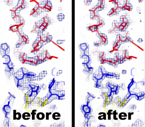 The second way anisotropy impacts the R-factor is by
degrading the appearance of electron density maps, thus
impeding model building attempts. In the case cited above (Strong et al.,
2006), the main chain electron density lacked carbonyl bumps and side
chain density appeared as blobs, despite the use of 2.3 Angstrom resolution
data. (See "before" panel at left.) As a consequence, it was difficult to determine
whether the chain was traced correctly and there was no indication
of any ordered water molecules in the map. After much analysis, it
was discovered that this lack of detail could be traced to the
automatically applied anisotropic scaling algorithm in REFMAC and CNS.
These algorithms eliminate anisotropy from the data set by
applying resolution dependent scale factors (equivalent to
B-factors) to three principle directions of the data set, so that the
magnitude of the structure factors decreases with resolution at equal
rates in all three dimensions. In effect, the magnitude of the
reflections in the weakly diffracting direction are scaled up while the
magnitude of the reflections in the strongly diffracting direction are
scaled down. The unwanted side effect of this procedure is that the high
resolution reflections in the strongly diffracting direction of the
crystal are diminished to the point that they
contribute very little to the electron density map; hence, the lack of
detail in the map. The solution used to correct this aspect of the problem is
to apply a negative isotropic B-factor to the data set to restore
the magnitude of the high resolution reflections to their original values.
As a result, the electron density maps improved immensely in detail
(see "after" panel at left) and Rwork and Rfree dropped approximately 13%
each, to their final values 24.7% and 31.2%, respectively.
The second way anisotropy impacts the R-factor is by
degrading the appearance of electron density maps, thus
impeding model building attempts. In the case cited above (Strong et al.,
2006), the main chain electron density lacked carbonyl bumps and side
chain density appeared as blobs, despite the use of 2.3 Angstrom resolution
data. (See "before" panel at left.) As a consequence, it was difficult to determine
whether the chain was traced correctly and there was no indication
of any ordered water molecules in the map. After much analysis, it
was discovered that this lack of detail could be traced to the
automatically applied anisotropic scaling algorithm in REFMAC and CNS.
These algorithms eliminate anisotropy from the data set by
applying resolution dependent scale factors (equivalent to
B-factors) to three principle directions of the data set, so that the
magnitude of the structure factors decreases with resolution at equal
rates in all three dimensions. In effect, the magnitude of the
reflections in the weakly diffracting direction are scaled up while the
magnitude of the reflections in the strongly diffracting direction are
scaled down. The unwanted side effect of this procedure is that the high
resolution reflections in the strongly diffracting direction of the
crystal are diminished to the point that they
contribute very little to the electron density map; hence, the lack of
detail in the map. The solution used to correct this aspect of the problem is
to apply a negative isotropic B-factor to the data set to restore
the magnitude of the high resolution reflections to their original values.
As a result, the electron density maps improved immensely in detail
(see "after" panel at left) and Rwork and Rfree dropped approximately 13%
each, to their final values 24.7% and 31.2%, respectively.
For more background on diffraction anisotropy and how it was corrected in (Strong et al., 2006), please see the following PowerPoint presentation presented by Michael Sawaya at the 2006 ACA meeting. | |||||
| Service Provided by the Diffraction Anisotropy Server | |||||
 The server indicates the severity of anisotropy in your data set.
The degree of anisotropy is indicated by the anisotropic delta
B statistic. It is the first statistic reported when you submit
your data to the diffraction anisotropy server. It measures the
directional dependence of the intensity falloff with resolution.
The directionality is paramaterized by three principle components
(analogous to B-factors), one for each direction of the crystal. (In an
orthorhombic crystal, these directions would correspond to a*, b*, and c*.)
If the falloff is nearly the same in all three directions, the three
principle components will be approximately equal and close to zero. If
the falloff has a strong directional dependence, then the component
describing the weakest diffracting direction will be large and positive
and the component describing the strongest diffracting direction will be
large and negative. Regardless of the degree of anisotropy, the sum of
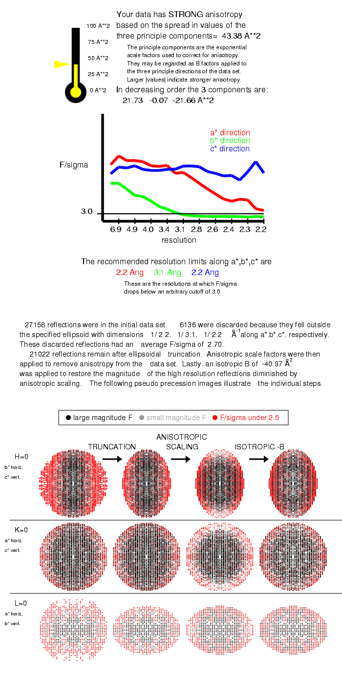
the three components are constrained to add up to zero. The anisotropic delta-B is defined
as the difference between the two components with the most extreme values.
An anisotropic delta-B of 10 Angstroms^2 indicates mild anisotropy.
An anisotropic delta-B over 25 Angstroms^2 indicates strong anisotropy.
An anisotropic delta-B over 50 Angstroms^2 indicates severe anisotropy.
The stronger the anisotropy, the more beneficial it is to employ the
ellipsodal truncation and anisotropic scaling performed by the server.
The example shown at right is taken from the data set described in
(Strong et al., 2006).
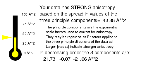
The server indicates the severity of anisotropy in your data set.
The degree of anisotropy is indicated by the anisotropic delta
B statistic. It is the first statistic reported when you submit
your data to the diffraction anisotropy server. It measures the
directional dependence of the intensity falloff with resolution.
The directionality is paramaterized by three principle components
(analogous to B-factors), one for each direction of the crystal. (In an
orthorhombic crystal, these directions would correspond to a*, b*, and c*.)
If the falloff is nearly the same in all three directions, the three
principle components will be approximately equal and close to zero. If
the falloff has a strong directional dependence, then the component
describing the weakest diffracting direction will be large and positive
and the component describing the strongest diffracting direction will be
large and negative. Regardless of the degree of anisotropy, the sum of
the three components are constrained to add up to zero. The anisotropic delta-B is defined
as the difference between the two components with the most extreme values.
An anisotropic delta-B of 10 Angstroms^2 indicates mild anisotropy.
An anisotropic delta-B over 25 Angstroms^2 indicates strong anisotropy.
An anisotropic delta-B over 50 Angstroms^2 indicates severe anisotropy.
The stronger the anisotropy, the more beneficial it is to employ the
ellipsodal truncation and anisotropic scaling performed by the server.
The example shown at right is taken from the data set described in
(Strong et al., 2006).
 The server recommends resolution limits for the 3 principle axes of the ellipsoid.
F/sigma is plotted for the three princple directions of the crystal
(red, green, blue). The resolutions at which F/sigma drops below 3.0
for each of the 3 principle axes are selected by default
as the resolution limits for ellipsoidal truncation. The example shown here
on the left is taken from the data set described in
(Strong et al., 2006). In this case, the recommended resolution limits
would be 2.2 Angstroms along the a*
direction, 3.1 Angstroms along the b* direction, and 2.2 Angstroms along
the c* direction. If you dont agree with this criteria, you may chose
your own limits, enter them in the server, and peform the ellipsoidal
truncation again. User input values override the recommended values.
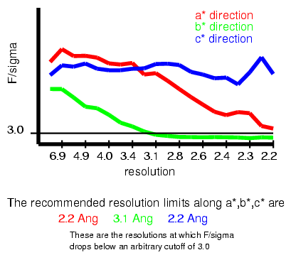
The server recommends resolution limits for the 3 principle axes of the ellipsoid.
F/sigma is plotted for the three princple directions of the crystal
(red, green, blue). The resolutions at which F/sigma drops below 3.0
for each of the 3 principle axes are selected by default
as the resolution limits for ellipsoidal truncation. The example shown here
on the left is taken from the data set described in
(Strong et al., 2006). In this case, the recommended resolution limits
would be 2.2 Angstroms along the a*
direction, 3.1 Angstroms along the b* direction, and 2.2 Angstroms along
the c* direction. If you dont agree with this criteria, you may chose
your own limits, enter them in the server, and peform the ellipsoidal
truncation again. User input values override the recommended values.
The server performs ellipsoidal truncation. Reflections falling outside the ellipsoid defined by the three specified resolution limits will be discarded from the data set. The result of the truncation is illustrated in a zero level pseudo precession image. Panels A and B below illustrate the ellipsoidal truncation procedure for the data set described in (Strong et al., 2006). Specifically, the h=0 plane is illustrated. Structure factor magnitudes are plotted in grayscale, with the largest |F|s represented in black. Structure factors with F/sigma less than 2.5 are highlighted in red. The server reports the number of reflections discarded and the average F/sigma of these reflections. If the limits are chosen correctly, the F/sigma will be less than 3.0 and the majority of the red colored reflections will have been removed, as appears to be the case here. In detail, 27158 reflections were in the initial data set. 6136 reflections were discarded because they fell outside the ellipsoid specified by resolution limits 2.2, 3.1, and 2.2 Angstroms along a*, b*, and c*. These discarded reflections had an average F/sigma of 2.70. 21022 reflections remain after ellipsoidal truncation. The truncation algorithm is rather straightforward, for details see the following PowerPoint presentation. 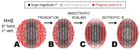 The server performs anisotropic scaling.
Anisotropy is removed from the data by anisotropic scaling.
The result is a nominally isotropic data set in which the slope
of |F| vs. resolution is equal in all directions.
Panel C illustrates the anisotropic scaling procedure for the
data set described in
(Strong et al., 2006).
Note that |F|/sigma|F| does not change in
this procedure. |F| and the sigma|F| are scaled by the same
multiplicative constant.
The server performs anisotropic scaling.
Anisotropy is removed from the data by anisotropic scaling.
The result is a nominally isotropic data set in which the slope
of |F| vs. resolution is equal in all directions.
Panel C illustrates the anisotropic scaling procedure for the
data set described in
(Strong et al., 2006).
Note that |F|/sigma|F| does not change in
this procedure. |F| and the sigma|F| are scaled by the same
multiplicative constant.
The server applies a negative isotropic B-factor correction. A negative isotropic B-factor is applied to the data set to restore the magnitude of the high resolution reflections to their original values (i.e. before the anisotropic scaling procedure). Comparison of panels B and C illustrates the need for the negative isotropic B-factor correction. Notice in panel C, that the high resolution reflections near the vertical axis were diminished by the anisotropic scaling procedure (i.e. they appear lighter gray compared to panel B). In panel D, these reflections are restored to their former magnitude as evidenced by comparing the similarity in darkness of these reflections in panel B and D. The server provides the corrected structure factors. A link to an MTZ format file containing the corrected structure factors will appear. These corrected structure factors may be used to continue crystallographic refinement as normal. Example output from anisotropy server. Diffraction Anisotropy Server program schematic. This principle components analysis and isotropic scaling was implemented with the program "phaser" available from Randy Read's Group The Anisotropy falloff plot is generated with the aid of the program "truncate" from the CCP4 suite of crystallographic programs. To report Rmerge statistics after ellipsoidal truncation, ellipsoidal truncation must be performed on UNMERGED data. Unfortunately, the version of the anisotropy server offered on this page cannot accept unmerged .mtz files. However, if you processed your data with Denzo/Scalepack, you can perform ellipsoidal truncation on your .x files using the special .x-files version of the ellipsoidal truncation program that you can download here. Then run Scalepack on the truncated .x files to get Rmerge statistics. After downloading the file, uncompressing it and untar-ing it, read the README file for instructions.If your data is processed with XDS/XSCALE, then use the XDS version of the server . It can be run over the web. You won't have to download any programs. You will get a table with all the data collection statistics before and after ellipsoidal truncation (Rmerge, completeness, and I/sigma). |
Comments and Questions on the Anisotropy Server may be sent to: sawaya@mbi.ucla.edu
Please send any Problems with the website to: holton@mbi.ucla.edu